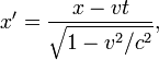
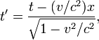
Ранее мы уже изучили формулы, называемые классическими преобразованиями Галилея, однако они несовместимы с постулатами специальной теории относительности (СТО). Поэтому в данном случае нам нужно использовать другие положения. Благодаря новым преобразованиям мы сможем установить, какая связь существует между некоторым моментом события t, наблюдаемого в системе отсчета K в точке с координатами (x, y, z) и показателями того же события, которое наблюдается в системе отсчета K’.
Преобразования Лоренца представляют собой кинематические формулы, с помощью которых происходит преобразование координат и времени в специальной теории относительности.
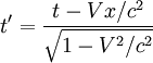
Они были впервые сформулированы еще в 1904 году в качестве преобразований, относительно которых были инвариантны уравнения электродинамики.
Обозначим основные системы K и K’, скорость их движения – υ, а ось, вдоль которой они движутся – x. В таком случае преобразования Лоренца примут следующий вид:
K’→Kx=x’+υt’1-β2,y=y’,z=z’,t=t’+υx’/c21-β2. K→K’x’=x-υt1-β2,y’=y,z’=z,t’=t-υx/c21-β2.
β=υc.
Используя эти формулы, мы можем вывести из них множество следствий. Так, именно из системы преобразований Лоренца следует лоренцево сокращение длины и релятивистский эффект замедления времени.
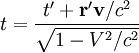
Возьмем случай, когда в системе K’ происходит некий процесс, длительность которого составляет τ0 = t’2 – t’1 (по собственному времени). Здесь t’1 и t’2 – это время на часах в начале данного процесса и в его конце. Чтобы вычислить его общую продолжительность в точке x, необходимо взять для расчета следующую формулу:
τ=t2-t1=t’2+υx’/c21-β2-t’1+υx’/c21-β2=t’2-t’11-β2=τ01-β2.
Формула релятивистского сокращения длины выводится из преобразований Лоренца точно таким же образом.
Принцип относительности одновременности
Еще одно важное следствие, которое необходимо знать, – это положение о том, что любая одновременность относительна.
Например, если в системе отсчета K’ взять две разные точки, в которых некий процесс будет протекать одновременно (с позиции стороннего наблюдателя), то в системе наблюдатель будет иметь следующее:
x1=x’1+υt’1-β2, x2=x’2+υt’1-β2⇒x1≠x2,t1=t’+υx’1/c21-β2, t2=t’+υx’2/c21-β2⇒t1≠t2.
Из этого вытекает пространственная разобщенность данных событий в системе K, следовательно, они не могут считаться одновременными. Нельзя сразу сказать, какое событие будет происходить первым, а какое вторым, поскольку это определяется особенностями системы отсчета – знак разности будет определен знаком выражения υ(x’2–x’1).
Если между событиями имеется причинно-следственная связь, то данный вывод специальной теории относительности для них использовать нельзя. Однако мы можем показать, что при этом не нарушается принцип причинности, и события следуют в нужном порядке в любой инерциальной системе отсчета.
Разберем пример, показывающий, что одновременность разобщенных в пространстве событий является относительной.
Возьмем систему отсчета K’ и расположим в ней длинный жесткий стержень. Его положение будет неподвижным и ориентированным вдоль оси абсцисс. Установим на оба его конца часы, синхронизированные между собой, а в центр поместим импульсную лампу. Также у нас будет система K’, совершающая движение вдоль оси x в системе K.
В определенный момент времени лампа включится и пошлет световые сигналы в направлении обоих концов жесткого стержня. Поскольку она находится точно в центре, эти сигналы должны дойти до концов в одно и то же время t, которое должно быть зафиксировано расположенными на них часами. Однако концы стержня движутся относительно системы K так, что один конец стремится навстречу световому сигналу, а другой конец свету приходится догонять. Скорость света, распространяющегося в оба направления, одинакова, но сторонний наблюдатель скажет, что до левого конца свет дошел быстрее, чем до правого.

Рисунок 4.4.1. Иллюстрация принципа относительности одновременности: достижение световым импульсом концов стержня в системе K’ в одно и то же время и в системе K в разное.
Инвариантные величины в СТО
Данные преобразования нужны нам для выражения относительного характера временных промежутков и промежутков расстояний. Вместе с тем в специальной теории относительности помимо утверждения относительного характера времени и пространства очень важно установить инвариантные физические величины, не изменяющиеся при смене системы отсчета. Подобной величиной является скорость света в вакууме, чей характер в рамках СТО становится абсолютным. Также важна такая величина, как интервал между событиями, поскольку именно она выражает абсолютность пространственно-временной связи.
Для вычисления пространственно-временного интервала необходимо использовать следующую формулу:
s12=c2t122-l122.
В ней с помощью параметра l12 выражено расстояние между точками одной системы, где совершаются события, а t12 – это временной промежуток между теми же самыми событиями. Если местом одного из событий является начало координат, т.е. x1=y1=z1=0 и (t1=0), а второе происходит в точке с координатами x, y, z в некоторое время t, то формула вычисления пространственно-временного интервала между ними записывается так:
s=c2t2-x2-y2-z2.
Преобразования Лоренца дают нам возможность доказать неизменность пространственно-временного интервала между событиями при смене инерциальной системы.
Если величина интервала не зависит от того, какая система отсчета используется, т.е. является объективной при любых относительных расстояниях и временных промежутках, то такой интервал называется инвариантным.
Допустим, что у нас есть событие (вспышка света), которое произошло в точке начала координат в некоторой системе во время, равное 0, а потом свет переместился в другую точку с координатами x, y, z во время t. Тогда мы можем записать следующее:
x2+y2+z2=c2t2.
У нас получилось, что интервал этой пары событий будет равен нулю. Если мы поменяем систему координат и возьмем другое время для второго события, то результаты окажутся точно такими же, поскольку:
x2+y2+z2=c2t2
Иначе говоря, любые два события, которые связывает между собой световой сигнал, будут иметь нулевой пространственно-временной интервал.
Также формулы Лоренца для времени и координат можно использовать для выведения релятивистского закона сложения скоростей.
Например, у нас есть частица, которая находится в системе отсчета K’ и движется в ней вдоль оси абсцисс со скоростью u’x=dx’dt’. Параметры скорости u’x и u’ равны 0. В системе K, соответственно, скорость будет равна ux=dxdt.
Применим к одной из формул преобразования Лоренца операцию дифференцирования и получим следующее:
ux=u’x+υ1+υc2u’x, uy=0, uz=0.
Данные отношения являются выражением релятивистского закона сложения скоростей. Он применим в случае движения частицы параллельно относительной скорости υ→ в системах отсчета K и K’.
Если υ≪c, то релятивистские отношения могут быть преобразованы в формулы классической механики:
ux=u’x+υ, uy=0, uz=0.
Если мы имеем дело со световым импульсом, распространяющимся в системе K’ вдоль оси x’ со скоростью u’x=c, то в этом случае применима следующая формула:
ux=c+υ1+υ/c=c, uy=0, uz=0.
Иначе говоря, скорость распространения светового импульса в системе K вдоль оси x также будет равна c, что соответствует постулату об инвариантности скорости света.
Преобразования Лоренца
Преобразова́ния
Ло́ренца — линейные (или аффинные)
преобразования векторного (соответственно,
аффинного) псевдоевклидова
пространства, сохраняющее длины
или, что эквивалентно, скалярное
произведение векторов.
Преобразования
Лоренца псевдоевклидова пространства
сигнатуры
(n-1,1) находят широкое применение в физике,
в частности, в специальной
теории относительности (СТО),
где в качестве аффинного псевдоевклидова
пространства выступает
четырёхмерный пространственно-временной
континуум (пространство
Минковского).
Преобразования Лоренца в физике
Преобразованиями
Лоренца в физике, в частности, в специальной
теории относительности (СТО),
называются преобразования, которым
подвергаются пространственно-временные
координаты (x,y,z,t) каждого
события при переходе от одной инерциальной
системы отсчета (ИСО) к другой.
Аналогично, преобразованиям Лоренца
при таком переходе подвергаются
координаты любого 4-вектора.
Чтобы
явно различить преобразования Лоренца
со сдвигами начала отсчёта и без сдвигов,
когда это необходимо, говорят о
неоднородных и однородных
преобразованиях Лоренца.
Преобразования
Лоренца без сдвигов начала отсчёта
образуют группу
Лоренца, со сдвигами — группу
Пуанкаре, иначе называемую
неоднородной группой Лоренца.
С
математической точки зрения преобразования
Лоренца — это преобразования,
сохраняющие неизменной метрику
Минковского, то есть, в частности,
последняя сохраняет при них простейший
вид при переходе от одной инерциальной
системы отсчёта к другой (другими словами
преобразования Лоренца — это аналог
для метрики Минковского ортогональных
преобразований, осуществляющих переход
от одного ортонормированного базиса к
другому, то есть аналог поворота
координатных осей для пространства-времени).
В математике или теоретической физике
преобразования Лоренца могут относиться
к любой размерности пространства.
Именно
преобразования Лоренца, смешивающие —
в отличие от преобразований
Галилея — пространственные
координаты и время, исторически стали
основой для формирования концепции
единого пространства-времени.
-
Следует заметить, что лоренц-ковариантны
не только фундаментальные уравнения
(такие, как уравнения Максвелла,
описывающее электромагнитное поле,
уравнение Дирака, описывающее электрон
и другие фермионы), но и такие
макроскопические уравнения, как волновое
уравнение, описывающее (приближенно)
звук, колебания струн и мембран, и
некоторые другие (только тогда уже в
формулах преобразований Лоренца под
c следует иметь в виду не скорость
света, а какую-то другую константу,
например скорость звука). Поэтому
преобразования Лоренца могут быть
плодотворно использованы и в связи с
такими уравнениями (хотя и в довольно
формальном смысле, впрочем, мало
отличающемся — в своих рамках —
от их применения в фундаментальной
физике).
Вид преобразований при коллинеарных (параллельных) пространственных осях
Если
ИСО K‘ движется относительно ИСО K
с постоянной скоростью v вдоль оси
x, а начала
пространственных координат
совпадают в начальный момент времени
в обеих системах, то преобразования
Лоренца (прямые) имеют вид:
![]()
![]()
где
c — скорость
света, величины со штрихами
измерены в системе K‘, без штрихов —
в K.
Эта
форма преобразования (то есть при выборе
коллинеарных осей), называемая иногда
бустом (англ. boost)
или лоренцевским бустом (особенно
в англоязычной литературе), несмотря
на свою простоту, включает, по сути, всё
специфическое физическое содержание
преобразований Лоренца, так как
пространственные оси всегда можно
выбрать таким образом, а при желании
добавить пространственные повороты не
представляет трудности (см. это в явном
развёрнутом виде ниже), хотя и делает
формулы более громоздкими.
-
Формулы, выражающие обратное
преобразование, то есть выражающие
x‘,y‘,z‘,t‘ через x,y,z,t
можно получить просто заменой v на
− v (абсолютная величина относительной
скорости движения систем отсчёта | v
| одинакова при измерении её в обеих
системах отсчёта, поэтому можно при
желании снабдить v штрихом, только
при этом надо внимательно следить за
тем, чтобы знак и определение
соответствовали друг другу) и взаимной
заменой штрихованных x и t с
нештрихованными. Или решая систему
уравнений (1) относительно x‘,y‘,z‘,t‘. -
Надо иметь
в виду, что в литературе преобразования
Лоренца часто записывается для упрощения
в системе единиц, где c = 1, что
действительно делает их вид более
изящным. -
Видно,
что при преобразованиях Лоренца события,
одновременные
в одной системе отсчёта, не являются
одновременными в другой (относительность
одновременности), кроме того, у движущегося
тела сокращается продольный размер по
сравнению с тем, какой оно имеет в
сопутствующей ему системе отсчёта
(лоренцево
сокращение), а ход движущихся
часов замедляется, если наблюдать их
из «неподвижной» системы отсчёта
(релятивистское
замедление времени).
Соседние файлы в предмете [НЕСОРТИРОВАННОЕ]
- #
- #
- #
- #
- #
- #
- #
- #
- #
- #
- #
Преобразованиями Лоренца в физике, в частности в специальной теории относительности (СТО), называются преобразования, которым подвергаются пространственно-временные координаты (x,y,z,t) каждого события при переходе от одной инерциальной системы отсчета (ИСО) к другой. Аналогично преобразованиям Лоренца при таком переходе подвергаются координаты любого 4-вектора.
Чтобы явно различить преобразования Лоренца со сдвигами начала отсчёта и без сдвигов, когда это необходимо, говорят о неоднородных и однородных преобразованиях Лоренца.
Преобразования Лоренца без сдвигов начала отсчёта образуют группу Лоренца, со сдвигами — группу Пуанкаре, иначе называемую неоднородной группой Лоренца.
С математической точки зрения преобразования Лоренца — это преобразования, сохраняющие неизменной метрику Минковского, то есть, в частности, последняя сохраняет при них простейший вид при переходе от одной инерциальной системы отсчёта к другой (другими словами преобразования Лоренца — это аналог для метрики Минковского ортогональных преобразований, осуществляющих переход от одного ортонормированного базиса к другому, то есть аналог поворота координатных осей для пространства-времени). В математике или теоретической физике преобразования Лоренца могут относиться к любой размерности пространства.
Именно преобразования Лоренца, смешивающие — в отличие от преобразований Галилея — пространственные координаты и время, исторически стали основой для формирования концепции единого пространства-времени.
- Следует заметить, что лоренц-ковариантны не только фундаментальные уравнения (такие, как уравнения Максвелла, описывающее электромагнитное поле, уравнение Дирака, описывающее электрон и другие фермионы), но и такие макроскопические уравнения, как волновое уравнение, описывающее (приближенно) звук, колебания струн и мембран, и некоторые другие (только тогда уже в формулах преобразований Лоренца под c следует иметь в виду не скорость света, а какую-то другую константу, например скорость звука). Поэтому преобразования Лоренца могут быть плодотворно использованы и в связи с такими уравнениями (хотя и в довольно формальном смысле, впрочем, мало отличающемся — в своих рамках — от их применения в фундаментальной физике).
Содержание
- 1 Вид преобразований при коллинеарных (параллельных) пространственных осях
- 2 Вывод преобразований
- 2.1 Алгебраический вывод
- 2.2 Группа симметрий уравнений Максвелла
- 2.3 Наглядный вывод преобразований Лоренца
- 2.3.1 Преобразование для поперечных осей (п.1)
- 2.3.2 Замедление времени (п.2)
- 2.3.3 Относительность одновременности (п.3)
- 2.3.4 Лоренцевское сокращение длины (п.4)
- 3 Разные формы записи преобразований
- 3.1 Вид преобразований при произвольной ориентации осей
- 3.2 Преобразования Лоренца в матричном виде
- 4 Свойства преобразований Лоренца
- 5 Связанные определения
- 6 История
- 7 Примечания
- 8 Литература
- 9 См. также
Вид преобразований при коллинеарных (параллельных) пространственных осях
Если ИСО K‘ движется относительно ИСО K с постоянной скоростью V вдоль оси x, а начала пространственных координат совпадают в начальный момент времени в обеих системах, то преобразования Лоренца (прямые) имеют вид:
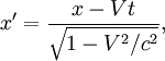


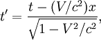
где c — скорость света в вакууме, величины со штрихами измерены в системе K‘, без штрихов — в K.
Эта форма преобразования (то есть при выборе коллинеарных осей), называемое иногда бустом (англ. boost) или лоренцевским бустом (особенно в англоязычной литературе), несмотря на свою простоту включает, по сути, всё специфическое физическое содержание преобразований Лоренца, так как пространственные оси всегда можно выбрать таким образом, а при желании добавить пространственные повороты не представляет трудности (см. это в явном развёрнутом виде ниже), хотя и делает формулы более громоздкими.
- Формулы, выражающие обратное преобразование, то есть выражающие x‘,y‘,z‘,t‘ через x,y,z,tможно получить просто заменой V на − V (абсолютная величина относительной скорости движения систем отсчёта | V | одинакова при измерении её в обеих системах отсчёта, поэтому можно при желании снабдить V штрихом, только при этом надо внимательно следить за тем, чтобы знак и определение соответствовали друг другу) и взаимной заменой штрихованных x и t с нештрихованными. Или решая систему уравнений (1) относительно x’, y’, z’, t’.
- Надо иметь ввиду, что в литературе преобразования Лоренца часто записывается для упрощения в системе единиц, где c = 1, что действительно делает их вид более изящным.
- Видно, что при преобразованиях Лоренца события, одновременные в одной системе отсчёта, не являются одновременными в другой (относительность одновременности), кроме того у движущегося тела сокращается продольный размер по сравнению с тем, какой оно имеет в сопутствующей ему системе отсчёта (лоренцево сокращение), а ход движущихся часов замедляется, если наблюдать их из «неподвижной» системы отсчёта (релятивистское замедление времени).
Вывод преобразований
Преобразования Лоренца могут быть получены абстрактно, из групповых соображений (в этом случае они получаются с неопределённым c), как обобщение преобразований Галилея (что было проделано Пуанкаре — см. ниже). Однако впервые были получены как преобразования, относительно которых ковариантны уравнения Максвелла (то есть по сути — которые не меняют законов электродинамики и оптики). Могут также быть получены из предположения линейности преобразований и постулата одинаковости скорости света во всех системах отсчёта (являющегося упрощённой формулировкой требования ковариантности электродинамики относительно искомых преобразований, и распространением принципа равноправия инерциальных систем отсчёта — принципа относительности — на электродинамику), как это делается в специальной теории относительности (СТО) (при этом c в преобразованиях Лоренца получается определённым и совпадает со скоростью света).
Надо заметить, что если не ограничивать класс преобразований координат линейными, то первый закон Ньютона выполняется не только для преобразований Лоренца, а для более широкого класса дробно-линейных преобразований (однако этот более широкий класс преобразований — за исключением, конечно, частного случая преобразований Лоренца — не сохраняет метрику постоянной).
Алгебраический вывод
На основании нескольких естественных предположений (основным из которых является предположение о существовании принципиально максимальной скорости распространения взаимодействий) можно показать, что при смене ИСО должна сохраняться величина
- ds2 = c2dt2 − dx2 − dy2 − dz2,
называемая интервалом. Из этой теоремы напрямую следует общий вид преобразований Лоренца (см. ниже). Здесь рассмотрим лишь частный случай. Для наглядности при переходе в ИСО K‘, движущуюся со скоростью v, выберем в исходной системе K ось X сонаправленной с v, а оси Y и Z расположим перпендикулярно оси X. Оси ИСО K‘ выберем сонаправленными с осями ИСО K. При таком преобразовании

Мы будем искать линейные преобразования Лоренца, так как при бесконечно малых преобразованиях координат дифференциалы новых координат линейно зависят от дифференциалов старых координат, а в силу однородности пространства и времени коэффициенты не могут зависеть от координат, только от взаимной ориентации и скорости ИСО.
То, что поперечные координаты не могут меняться, ясно из соображений изотропности пространства. Действительно, величина y‘ не может изменяться и при этом не зависеть от x (кроме как при вращении вокруг v, которое мы исключаем из рассмотрения), в чём легко убедиться подстановкой таких линейных преобразований в выражение для интервала. Но если она зависит от x, то точка с координатой (0,x,0,0) будет иметь ненулевую координату y‘, что противоречит наличию симметрии вращения системы относительно v и изотропии пространства. Аналогично для z‘.
Наиболее общий вид таких преобразований:

где α — некоторый параметр, называемый быстротой. Обратные преобразования имеют вид

Ясно, что точка, покоящаяся в ИСО K, должна будет двигаться в ИСО K‘ со скоростью − v. С другой стороны, если точка покоится, то

Учитывая, что при смене ИСО не должна меняться ориентация пространства, получим что

Следовательно, уравнение для быстроты однозначно разрешимо:
а преобразования Лоренца имеют вид
Параметр γ называется лоренц-фактором.
Группа симметрий уравнений Максвелла
Наглядный вывод преобразований Лоренца
Примем постулаты СТО, сводящиеся к расширенному принципу относительности, утверждающему, что все физические процессы протекают в точности одинаково во всех инерциальных системах отсчета (уточняющий его принцип постоянства скорости света в СТО означает расширение принципа относительности на электродинамику вместе с уточняющим утверждением о том, что нет никакой фундаментальной физической среды (эфира), которая выделяла бы одну из систем отсчета на опыте — то есть если даже эфир и есть, то его наличие не должно никак нарушать принципа относительности на практике). Кроме того, полезно явно подчеркнуть, что принцип постоянства скорости света означает наличие именно конечной скорости (скорости света), заложенной в фундаментальные законы (уравнения), одной и той же для всех инерциальных систем отсчета, причём и в каждой системе отсчета величина скорости света одинакова для любых направлений его распространения (это используется ниже).
Преобразование для поперечных осей (п.1)
Пусть есть две бесконечные плоскости, перпендикулярные оси y. Расстояние между этими плоскостями очевидно не должно зависеть от скорости движения плоскостей вдоль самих себя (то есть переходя в себя же), а значит — не зависит от выбора системы отсчета среди движущихся вдоль оси x. (Чтобы быть совсем уверенным в этом, можно провести мысленный эксперимент, заключающийся в измерении времени, требующегося лучу света, движущемуся вдоль y в каждой такой системе отсчета, для того, чтобы, стартовав на одной плоскости, достичь второй, и увидеть, что такое время очевидно будет одинаковым, если верны постулаты СТО).
То же самое, конечно, верно и для оси z. Поэтому, исключив для простоты физически неинтересный случай поворота координат второй системы относительно первой на постоянный (независящий от времени) угол, получаем:
- y = y‘,z = z‘
Замедление времени (п.2)
Показать, что любые процессы (например ход часов) выглядит медленнее из системы отсчета где носитель этого процесса (например часы) движется, чем в его собственной системе отсчета (в которой он неподвижен), и найти количественно фактор такого замедления, можно, рассмотрев мысленный эксперимент со «световыми часами», представляющими собой источник и приемник света, удаленные друг от друга на известное фиксированное расстояние L, и отмеряющие, таким образом, интервал времени L/c, соответствующий времени прохождения света от источника до приемника (это можно непрерывно повторять). Все другие часы, из принципу относительности, должны идти точно так же.
Для более прямого соответствия формы полученного результата формуле прямого преобразования Лоренца, будем считать, что наши световые часы покоятся в нештрихованой системе отсчета K, штрихованая же система отсчета K’ пусть движется для определенности вправо вдоль оси x со скоростью V. Источник и приемник расположим вдоль оси y при x=0. Это частный случай, который позволит нам получить сперва отдельно частное и более простое преобразование для времени.
Поместим источник в начальный момент времени в начало координат, обозначив его A (см. рисунок, там он изображен красной точкой), а приемник обозначим B (синяя точка). В нештрихованой системе отсчета (на рисунке слева) импульс света летит точно по оси y (B, как и A в этой системе неподвижны). Таким образом, от излучения до поглощения света в этой системе проходит время  .
.
В штрихованой же системе отсчета точки A и B движутся влево со скоростью V. Особенно нас интересует движение точки B, обозначенное на рисунке пунктиром. Из-за этого ее смещения, равного  , свету в этой системе отсчета приходится пройти не расстояние L, а большее (на рисунке путь света от A к B изображен зеленой линией). Это расстояние нетрудно выразить с помощью теоремы Пифагора, и оно же равно ct’, откуда:
- (ct‘)2 = L2 + (Vt‘)2,
а учитывая упомянутые чуть выше L = ct и выражая t’ через t, имеем:
 ,
,
 ,
,что и является преобразованием Лоренца для времени для условия x = 0.
(по сути же это есть замедление времени при наблюдении часов — или любого другого процесса с локальным носителем — из системы отсчета, движущейся относительно него: мы видим, что t’ > t).
Относительность одновременности (п.3)
Кроме замедления времени в движущейся системе отсчета (замедления хода всех часов движущейся лаборатории при наблюдении их из неподвижной), оказывается, что начало отсчета времени в движущейся системе отсчета также не совпадает с таковым в неподвижной, причем сдвиг этого начала отсчета — разный в разных точках — зависит от x (часы, выглядящие синхронными в своей собственной системе отсчета, выглядят идущими с разным опережением-отставанием, зависящим от их пространственного расположения, если на них смотреть из другой системы отсчета, такой, в которой их собственная система отсчета движется).
Чтобы стало понятным само существо проблемы, придется так или иначе обдумать вопрос, а что значит, что часы в разных удаленных друг от друга точках пространства (например, в разных городах) идут одинаково (синхронно), как в этом можно убедиться, или как (с помощью какой процедуры) можно синхронизировать часы в разных местах, если изначально они не были синхронны.
Уже простейший способ синхронизации, заключающийся в том, что все часы синхронизируют в одном месте, а затем переносят в разные точки, позволяет качественно убедиться в том, что часы, синхронизированные в одной системе отсчета, будут выглядеть показывающими разное время из другой системы отсчета. Дело в том, что для часов, которые мы переносим вправо по оси x и влево по оси x, — время будет замедляться по-разному, так как их скорость будет обязательно различной в этой другой системе отсчета.
Это можно было бы аккуратно рассмотреть количественно, получив так искомый здесь результат. Но более просто этого достичь позволяет рассмотрение синхронизации с помощью световых сигналов (а принцип относительности говорит, что любой корректный способ синхронизации должен дать один и тот же результат, в чём, впрочем, при желании можно убедиться и явно).
Итак, рассмотрим синхронизацию с помощью световых сигналов. Этот процесс может заключаться, например, в обмене световыми сигналами между двумя удаленными хронометрами: если сигналы испущены в одно и то же время, то до получения сигнала по каждым часам пройдет одно и то же время. Но еще проще несколько другой (эквивалентный этому) способ: можно точно в середине отрезка, соединяющего хронометры, произвести вспышку света, и утверждать, что свет придет к обоим хронометрам одновременно.
В собственной системе отсчета (в которой хронометры неподвижны) картина симметрична. Однако в любой другой системе отсчета оба хронометра движутся (для определенности будем считать, что вправо), и тогда свету от середины отрезка, соединяющего их в начальный момент, потребуется меньше времени, чтобы дойти до левого хронометра (движущегося навстречу свету), чем до правого (который импульс света должен догонять).
Таким образом, хронометры, синхронные в своей собственной системе отсчета, по часам другой системы отсчета выглядят несинхронными. А это и означает, что события, одновременные в одной системе отсчета, неодновременны в другой. Это и называется относительностью одновременности.
Несложные геометрические выкладки позволяют (изобразив движение световых импульсов и хронометров на плоскости xt), получить выражение для сдвига начала отсчета времени:
- − Vx / c2
- (для упрощения мы здесь рассматривали только часы, разнесенные вдоль оси x, но, конечно, всё может быть рассчитано и для общего случая).
Таким образом, сводя вместе результаты пунктов 1 и 2, получаем для преобразования времени
- .
 .
.Лоренцевское сокращение длины (п.4)
Рассмотрев движение светового импульса вдоль оси x (а не вдоль y, как было в п.1), и потребовав (на основании постулата одинаковости скорости света во всех инерциальных системах отсчёта), чтобы расстояние между двумя точками было всегда равно времени, за которое свет идёт от одной точки до другой, делённому на (константу) скорость света, можно получить фактор сокращения расстояний вдоль оси x, а учитывая, что смещение начала отсчёта − Vt очевидно, можно получить и преобразование для x:
- .
 .
.Однако ещё проще теперь понять, что x‘ выражается именно таким образом, заметив, что в плоскости x − ct график движения[1] импульса света должен быть прямой, наклонённой под 45° (из-за того, что скорость света — всегда c), а значит и масштаб по x и по ct должен быть одинаковым, а выражения в системе единиц c = 1 — симметричными.
- Таким образом достаточно наглядно получаются преобразования Лоренца при коллинеарных пространственных осях. Конечно, возможен и обратный порядок рассуждений: можно сначала получить преобразования Лоренца каким-то более абстрактным способом, например — одним из упомянутых в статье выше, а потом получить все эффекты, разобранные в этапах данного наглядного доказательства, в качестве простого формального следствия преобразований Лоренца.
Разные формы записи преобразований
Вид преобразований при произвольной ориентации осей
В силу произвольности введения осей координат, многие задачи можно свести к указанному случаю. Если же задача требует иного расположения осей, то можно воспользоваться формулами преобразований в более общем случае. Для этого радиус-вектор точки
- ,
 ,
,где  — орты, надо разбить на составляющую
  параллельную скорости и составляющую
  ей перпендикулярную
- .
 .
.Тогда преобразования получат вид
 ,
,
где  — абсолютная величина скорости,
  — абсолютная величина продольной составляющей радиус-вектора.
Эти формулы для случая параллельных осей, но с произвольно направленной скоростью, можно преобразовать к виду, впервые полученному Герглоцем:
- .
 .
.Обратите внимание, что самый общий случай, когда начала координат не совпадают в нулевой момент времени, здесь не приведён с целью экономии места. Его можно получить, добавив к преобразованиям Лоренца трансляцию (смещение начала координат).
Преобразования Лоренца в матричном виде
Для случая коллинеарных осей преобразования Лоренца записываются в виде
- ,
 ,
,где 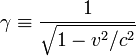 .
.
При произвольной ориентации осей, в форме 4-векторов это преобразование записывается как:
где E — единичная матрица 3 3,
3,  — тензорное умножение трехмерных векторов.
Надо иметь ввиду, что в литературе матрица преобразований Лоренца часто записывается для упрощения в системе единиц, где c = 1.
Произвольное однородное преобразование Лоренца можно представить как некоторую композицию вращений пространства и элементарных преобразований Лоренца, затрагивающих только время и одну из координат. Это следует из алгебраической теоремы о разложении произвольного вращения на простые.
Свойства преобразований Лоренца
- Можно заметить, что в случае, когда , преобразования Лоренца переходят в преобразования Галилея. То же самое происходит в случае, когда . Это говорит о том, что специальная теория относительности совпадает с механикой Ньютона либо в мире с бесконечной скоростью света, либо при скоростях, малых по сравнению со скоростью света. Последее объясняет, каким образом сочетаются эти две теории — первая является обобщением и уточнением второй, а вторая — предельным случаем первой, оставаясь в этом качестве верной приближенно (с некоторой точностью, на практике часто очень и очень большой) при достаточно малых (по сравнению со скоростью света) скоростях движений.
 , преобразования Лоренца переходят в преобразования Галилея. То же самое происходит в случае, когда
  . Это говорит о том, что специальная теория относительности совпадает с механикой Ньютона либо в мире с бесконечной скоростью света, либо при скоростях, малых по сравнению со скоростью света. Последее объясняет, каким образом сочетаются эти две теории — первая является обобщением и уточнением второй, а вторая — предельным случаем первой, оставаясь в этом качестве верной приближенно (с некоторой точностью, на практике часто очень и очень большой) при достаточно малых (по сравнению со скоростью света) скоростях движений.
- Преобразования Лоренца сохраняют инвариантным интервал для любой пары событий (точек пространства-времени) — то есть любой пары точек пространства — времени:

(убедиться в этом нетрудно, например, убедившись явно в том, что матрица преобразования Лоренца L — ортогональна в смысле метрики, определяемой таким выражением, то есть если  , что проще всего проверить для буста, для трехмерных же вращений это очевидно, следовательно, верно и для любых их композиций; как только мы узнали, что преобразования ортогональны, значит расстояние, вычисленное в такой метрике, неизменно в любой системе координат — по свойству ортогональных преобразований).
- В частности, инвариантность интервала имеет место и для случая s = 0, а значит — гиперповерхность в пространстве-времени, которая определяется равенством нулю интервала до заданной точки — световой конус — является неподвижной при преобразованиях Лоренца (что является проявлением инвариантности скорости света). Внутреность двух полостей конуса соответствует времениподобным — вещественным — интервалам от их точек до вершины, внешняя область — пространственноподобным — чисто мнимым (в принятой в этой статье сигнатуре интервала).
- Другие инвариантные гиперповерхности однородных преобразований Лоренца (аналоги сферы для пространства Минковского) — гиперболоиды: двуполостный гиперболоид для времениподобных интервалов относительно начала координат, и однополостный — для пространственноподобных интервалов.
- Матрицу преобразования Лоренца при коллинеарных пространственных осях (в системе единиц c=1) можно представить как:
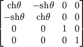
- где . В этом легко убедиться, учитывая и проверив выполнение соответствущего тождества для матрицы преобразования Лоренца в обычном виде.
 . В этом легко убедиться, учитывая
 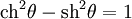 и проверив выполнение соответствущего тождества для матрицы преобразования Лоренца в обычном виде.
Связанные определения
Лоренц-инвариантность — свойство физических законов записываться одинаково во всех инерциальных системах отсчета(с учетом преобразований Лоренца). Принято считать, что этим свойством должны обладать все физические законы, и экспериментальных отклонений от него не обнаружено. Однако некоторые теории пока не удаётся построить так, чтобы выполнялась Лоренц-инвариантность.
История
Преобразования названы в честь их первооткрывателя — Х. А. Лоренца, который впервые ввел их (вместо преобразований Галилея) в качестве преобразований, связывающих геометрические величины (длины, углы), измеренных в разных инерциальных системах отсчета, чтобы устранить противоречия между электродинамикой и механикой, которые имелись в ньютоновской формулировке, включающей преобразования Галилея, что в конечном итоге привело к успеху при существенной модификации механики.
Сначала было обнаружено, что уравнения Максвелла инвариантны относительно этих преобразований (В. Фогтом в 1887 г.). Это же было повторено Лармором в 1900 г..
В 1892 г. Лоренц ввёл теорию сокращения, предполагающую сокращение длин всех твёрдых тел в направлении движения, количественно совпадающее с тем, что понимается сейчас под лоренцевым сокращением.
Преобразования Лоренца были впервые опубликованы в 1904 г. но в то время их форма была несовершенна. К современному, полностью самосогласованному виду их привёл французский математик А. Пуанкаре. Только в 1905 г. Пуанкаре и затем Эйнштейн в своей теории относительности пришёл к широко популярной впоследствии формально-аксиоматической трактовке этих преобразований. Пуанкаре же ввел термины «преобразования Лоренца» и «группа Лоренца», показал, исходя из эфирной модели, невозможность обнаружить движение относительно абсолютной системы отсчета (системы, в который эфир неподвижен), модифицировав таким образом принцип относительности Галилея. Ему же принадлежит групповой вывод явного вида преобразований Лоренца (с неопределенным c) без независимого постулата инвариантности скорости света.
Примечания
- ↑ Минковский назвал такой график движения мировой линией; однако в этом параграфе мы не будем углубляться в связь преобразований Лоренца с понятием пространства Минковского в полном его объёме, прежде всего — чтобы не усложнять и не прерывать элементарный вывод, который удобнее считать независимым от каких-либо дополнительных специальных понятий, ограничившись только элементарными геометрическими и алгебраическими понятиями лишь настолько, насколько они необходимы. По сути, речь идёт именно о преобразовании координат в пространстве Минковского, причём в данном параграфе, исходя из постулата постоянства скорости света, как раз и выясняются определённые свойства этого пространства, как и преобразований Лоренца — в качестве удобных преобразований координат в нём. Но ещё раз для ясности подчеркнем, что для самого вывода не нужно знать ничего кроме того, что явно сказано в основном тексте параграфа.
Литература
- Ландау, Л. Д., Лифшиц, Е. М. Теория поля. — Издание 7-е, исправленное. — М.: Наука, 1988. — 512 с. — («Теоретическая физика», том II). — ISBN 5-02-014420-7
- Физическая энциклопедия, т.2 — М.:Большая Российская Энциклопедия стр.608 и стр.609.
- Ф. И. Фёдоров Группа Лоренца. — М.: Наука, 1979. 384 с.
- Гельфанд И. М., Минлос Р. А., Шапиро З. Я. Представление группы вращений и группы Лоренца. М., 1958.
См. также
- Сложное движение (формула преобразования скорости, согласованная с преобразованиями Лоренца)
Wikimedia Foundation.
2010.
A visualisation of the Lorentz transformation (full animation). Only one space coordinate is considered. The thin solid lines crossing at right angles depict the time and distance coordinates of an observer at rest with respect to that frame; the skewed solid straight lines depict the coordinate grid of an observer moving with respect to that same frame.
In physics, the Lorentz transformation describes how, according to the theory of special relativity, two observers’ varying measurements of space and time can be converted into each other’s frames of reference. It is named after the Dutch physicist Hendrik Lorentz. It reflects the surprising fact that observers moving at different velocities may measure different distances, elapsed times, and even different orderings of events.
The Lorentz transformation was originally the result of attempts by Lorentz and others to explain how the speed of light was observed to be independent of the reference frame, and to understand the symmetries of the laws of electromagnetism. Albert Einstein later re-derived the transformation from his postulates of special relativity. The Lorentz transformation supersedes the Galilean transformation of Newtonian physics, which assumes an absolute space and time (see Galilean relativity). According to special relativity, this is a good approximation only at relative speeds much smaller than the speed of light.
If space is homogeneous, then the Lorentz transformation must be a linear transformation. Also, since relativity postulates that the speed of light is the same for all observers, it must preserve the spacetime interval between any two events in Minkowski space. The Lorentz transformation describes only the transformations in which the spacetime event at the origin is left fixed, so they can be considered as a hyperbolic rotation of Minkowski space. The more general set of transformations that also includes translations is known as the Poincaré group.
Lorentz transformation for frames in standard configuration
Standard configuration of coordinate systems for Lorentz transformations.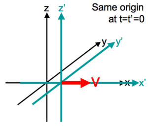
Assume there are two observers O and Q, each using their own Cartesian coordinate system to measure space and time intervals. O uses  and Q uses
  . Assume further that the coordinate systems are oriented so that the x-axis and the x’ -axis are collinear, the y-axis is parallel to the y’ -axis, as are the z-axis and the z’ -axis. The relative velocity between the two observers is v along the common x-axis. Also assume that the origins of both coordinate systems are the same. If all these hold, then the coordinate systems are said to be in standard configuration. A
symmetric presentation
between the forward Lorentz Transformation and the inverse Lorentz Transformation
can be achieved if coordinate systems are in
symmetric configuration.
The symmetric form highlights that all physical laws should be of such a kind that
they remain unchanged under a Lorentz transformation.
The Lorentz transformation for frames in standard configuration can be shown to be:

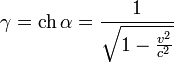
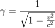
where  is called the Lorentz factor.
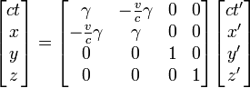
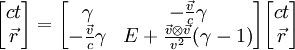
Matrix form
This Lorentz transformation is called a «boost» in the x-direction and is often expressed in matrix form as

This transformation matrix is universal for all four-vectors.
More generally for a boost in any arbitrary direction  ,
,

where  and
and  .
.
Note that this transformation is only the «boost,» i.e., a transformation between two frames whose  , and
, and  axis are parallel and whose spacetime origins coincide (see The «Standard configuration» Figure). The most general proper Lorentz transformation also contains a rotation of the three axes, because the composition of two boosts is not a pure boost but is a boost followed by a rotation. The rotation gives rise to Thomas precession. The boost is given by a symmetric matrix, but the general Lorentz transformation matrix need not be symmetric.
The composition of two Lorentz boosts B(u) and B(v) of velocities u and v is given by:
- ,
![{displaystyle B(mathbf {u} )B(mathbf {v} )=B(mathbf {u} oplus mathbf {v} )Gyr[mathbf {u} ,mathbf {v} ]=Gyr[mathbf {u} ,mathbf {v} ]B(mathbf {v} oplus mathbf {u} )}](https://wikimedia.org/api/rest_v1/media/math/render/png/9bf1d2551486450faf8eea070cef01473fecf1ef) ,
,where u v is the velocity-addition, and Gyr[u,v] is the rotation arising from the composition, gyr being the gyrovector space abstraction of the gyroscopic Thomas precession, and B(v) is the 4×4 matrix that uses the components of v, i.e. v1, v2, v3 in the entries of the matrix, or rather the components of v/c in the representation that is used above.
The composition of two Lorentz transformations L(u,U) and L(v,V) which include rotations U and V is given by:
![{displaystyle L(mathbf {u} ,U)L(mathbf {u} ,V)=L(mathbf {u} oplus Umathbf {v} ,gyr[mathbf {u} ,Umathbf {v} ]UV)}](https://wikimedia.org/api/rest_v1/media/math/render/png/0d3905fdc285619ed25882ae3b12808b0c59f13d)
If the 3×3 matrix form of the rotation applied to spatial coordinates is given by gyr[u,v], then the 4×4 matrix rotation applied to 4-coordinates is given by:
- .
![{displaystyle Gyr[mathbf {u} ,mathbf {v} ]={begin{pmatrix}1&0\0&gyr[mathbf {u} ,mathbf {v} ]end{pmatrix}}}](https://wikimedia.org/api/rest_v1/media/math/render/png/04b37c5747b7fa3dca29402cc362fe75037fbfa3) .
. Views of spacetime along the world line of a rapidly accelerating observer (center) moving in a 1-dimensional (straight line) «universe». The vertical direction indicates time, while the horizontal indicates distance, the dashed line is the spacetime trajectory («world line») of the observer. The small dots are specific events in spacetime. If one imagines these events to be the flashing of a light, then the events that pass the two diagonal lines in the bottom half of the image (the past light cone of the observer in the origin) are the events visible to the observer. The slope of the world line (deviation from being vertical) gives the relative velocity to the observer. Note how the view of spacetime changes when the observer accelerates.![]()
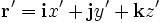
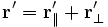
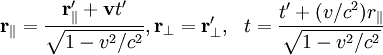
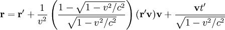
For a boost in an arbitrary direction with velocity  , it is convenient to decompose the spatial vector
  into components perpendicular and parallel to the velocity :
  . Then only the component
  in the direction of is ‘warped’ by the gamma factor:

where now  . The second of these can be written as:

These equations can be expressed in matrix form as

where I is the identity matrix, v is velocity written as a column vector, vT is its transpose (a row vector) and  is its versor.
Rapidity
The Lorentz transformation can be cast into another useful form by defining a parameter  called the rapidity (an instance of hyperbolic angle) such that

so that

Equivalently:
![{displaystyle phi =ln left[gamma (1+beta )right]=-ln left[gamma (1-beta )right],}](https://wikimedia.org/api/rest_v1/media/math/render/png/47a501800747e94121c6b8c882307d341bd63e8d)
Then the Lorentz transformation in standard configuration is:

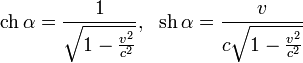
Hyperbolic trigonometric expressions
From the above expressions for eφ and e−φ


and therefore,

Hyperbolic rotation of coordinates
Substituting these expressions into the matrix form of the transformation, we have:

Thus, the Lorentz transformation can be seen as a hyperbolic rotation of coordinates in Minkowski space, where the rapidity  represents the hyperbolic angle of rotation, often referred to as rapidity.
Lorentz transformation of the electromagnetic field
The fact that the electromagnetic field shows relativistic effects becomes clear by carrying out a simple thought experiment:
- Consider an observer looking at a charge being at rest. The observer will find out that there is an electric field. Since there is no electric current, however, he will state not seing any magnetic field.
- If the observer moves toward or away from the charge with a certain velocity , he will notice that the electric field changes its value as a result of motion. This means, that he will measure different electric fields at the same place, depending on whether he is at motion or not. On the other hand, the observer will interpret the charge at motion as an electric current having a magnetic field around it.
This shows that electromagnetic field quantities need to undergo a Lorentz transformation when changing the frame of reference.
For the electric and magnetic field quantities, the following transformations apply :

In non-relativistic approximation, i. e. for speeds  , the relativistic factor
  equals
  , so that there is no need to distinguish between the spatial and temporal coordinates in Maxwell’s equations. This yields the following transformations:

The electric and magnetic fields transform differently from space and time, but exactly the same way as relativistic angular momentum and the boost vector.
The electromagnetic field strength tensor is given by

in SI units. In relativity, the Gaussian system of units is often preferred over SI units, even in texts whose main choice of units is SI units, because in it the electric field E and the magnetic induction B have the same units making the appearance of the electromagnetic field tensor more natural. Consider a Lorentz boost in the x-direction. It is given by

where the field tensor is displayed side by side for easiest possible reference in the manipulations below.
The general transformation law (T3) becomes

For the magnetic field one obtains

For the electric field results

Here, β = (β, 0, 0) is used. These results can be summarized by

and are independent of the metric signature. For SI units, substitute E → E⁄c. Misner, Thorne & Wheeler (1973) refer to this last form as the 3 + 1 view as opposed to the geometric view represented by the tensor expression

and make a strong point of the ease with which results that are difficult to achieve using the 3 + 1 view can be obtained and understood. Only objects that have well defined Lorentz transformation properties (in fact under any smooth coordinate transformation) are geometric objects. In the geometric view, the electromagnetic field is a six-dimensional geometric object in spacetime as opposed to two interdependent, but separate, 3-vector fields in space and time. The fields E (alone) and B (alone) do not have well defined Lorentz transformation properties. The mathematical underpinnings are equations (T1) and (T2) that immediately yield (T3). One should note that the primed and unprimed tensors refer to the same event in spacetime. Thus the complete equation with spacetime dependence is

Length contraction has an effect on charge density ρ and current density J, and time dilation has an effect on the rate of flow of charge (current), so charge and current distributions must transform in a related way under a boost. It turns out they transform exactly like the space-time and energy-momentum four-vectors,

or, in the simpler geometric view,

Spacetime interval
In a given coordinate system ( ), if two events
  and
and  are separated by

the spacetime interval between them is given by

This can be written in another form using the Minkowski metric. In this coordinate system,

Then, we can write

or, using the Einstein summation convention,

Now suppose that we make a coordinate transformation  . Then, the interval in this coordinate system is given by

or

It is a result of special relativity that the interval is an invariant. That is,  . It can be shown that this requires the coordinate transformation to be of the form

Here,  is a constant vector and
  a constant matrix, where we require that

Such a transformation is called a Poincaré transformation or an inhomogeneous Lorentz transformation. The  represents a spacetime translation. When
  , the transformation is called an homogeneous Lorentz transformation, or simply a Lorentz transformation.
Taking the determinant of  gives us

Lorentz transformations with  form a subgroup called proper Lorentz transformations which is the special orthogonal group
  . Those with
  are called improper Lorentz transformations which is not a subgroup, as the product of any two improper Lorentz transformations will be a proper Lorentz transformation. From the above definition of
  it can be shown that
  , so either
  or
or  , called orthochronous and non-orthochronous respectively. An important subgroup of the proper Lorentz transformations are the proper orthochronous Lorentz transformations which consist purely of boosts and rotations. Any Lorentz transform can be written as a proper orthochronous, together with one or both of the two discrete transformations; space inversion (
 ) and time reversal (
 ), whose non-zero elements are:


The set of Poincaré transformations satisfies the properties of a group and is called the Poincaré group. Under the Erlangen program, Minkowski space can be viewed as the geometry defined by the Poincaré group, which combines Lorentz transformations with translations. In a similar way, the set of all Lorentz transformations forms a group, called the Lorentz group.
A quantity invariant under Lorentz transformations is known as a Lorentz scalar.
Special relativity
One of the most astounding consequences of Einstein’s clock-setting method is the idea that time is relative. In essence, each observer’s frame of reference is associated with a unique set of clocks, the result being that time passes at different rates for different observers. This was a direct result of the Lorentz transformations and is called time dilation. We can also clearly see from the Lorentz «local time» transformation that the concept of the relativity of simultaneity and of the relativity of length contraction are also consequences of that clock-setting hypothesis.
Lorentz transformations can also be used to prove that magnetic and electric fields are simply different aspects of the same force — the electromagnetic force. If we have one charge or a collection of charges which are all stationary with respect to each other, we can observe the system in a frame in which there is no motion of the charges. In this frame, there is only an «electric field». If we switch to a moving frame, the Lorentz transformation will predict that a «magnetic field» is present. This field was initially unified in Maxwell’s concept of the «electromagnetic field».
The correspondence principle
For relative speeds much less than the speed of light, the Lorentz transformations reduce to the Galilean transformation in accordance with the correspondence principle.
The correspondence limit is usually stated mathematically as: as  ,
,  . In words: as velocity approaches 0, the speed of light (seems to) approach infinity. Hence, it is sometimes said that nonrelativistic physics is a physics of «instant action at a distance».
History
- See also History of Lorentz transformations.
Many physicists, including George FitzGerald, Joseph Larmor, Hendrik Lorentz and Woldemar Voigt, had been discussing the physics behind these equations since 1887.
Larmor and Lorentz, who believed the luminiferous ether hypothesis, were seeking the transformation under which Maxwell’s equations were invariant when transformed from the ether to a moving frame. Early in 1889, Oliver Heaviside had shown from Maxwell’s equations that the electric field surrounding a spherical distribution of charge should cease to have spherical symmetry once the charge is in motion relative to the ether. FitzGerald then conjectured that Heaviside’s distortion result might be applied to a theory of intermolecular forces. Some months later, FitzGerald published his conjecture in Science to explain the baffling outcome of the 1887 ether-wind experiment of Michelson and Morley. This idea was extended by Lorentz
and Larmor
over several years, and became known as the FitzGerald-Lorentz explanation of the Michelson-Morley null result, known early on through the writings of Lodge, Lorentz, Larmor, and FitzGerald.
Their explanation was widely known before 1905.
Larmor is also credited to have been the first to understand the crucial time dilation property inherent in his equations.
In 1905, Henri Poincaré was the first to recognize that the transformation has the properties of a mathematical group,
and named it after Lorentz.
Later in the same year Einstein derived the Lorentz transformation under the assumptions of the principle of relativity and the constancy of the speed of light in any inertial reference frame,
obtaining results that were algebraically equivalent to
Larmor’s (1897) and Lorentz’s (1899, 1904), but with a different interpretation.
Paul Langevin (1911) said of the transformation:
- «It is the great merit of H. A. Lorentz to have seen that the fundamental equations of electromagnetism admit a group of transformations which enables them to have the same form when one passes from one frame of reference to another; this new transformation has the most profound implications for the transformations of space and time».
Derivation
The usual treatment is based on the invariance of the speed of light, as seen by the Michelson-Morley experiment. However, this is not necessarily the starting point: indeed (as is exposed, for example, in the second volume of the Course of Theoretical Physics by Landau and Lifshitz), what is really at stake is the locality of interactions: one supposes that the influence that one particle, say, exerts on another can not be transmitted instantaneously. Hence, there exists a theoretical maximal speed of information transmission which must be invariant, and it turns out that this speed coincides with the speed of light in vacuum. The need for locality in physical theories was already noted by Newton (see Koestler’s The Sleepwalkers), who considered the notion of an action at a distance «philosophically absurd» and believed that gravity must be transmitted by an agent (such as an interstellar aether) which obeys certain physical laws.
Michelson and Morley in 1887 designed an experiment, employing an interferometer and a half-silvered mirror, that was accurate enough to detect aether flow. The mirror system reflected the light back into the interferometer. If there were an aether drift, it would produce a phase shift and a change in the interference that would be detected. However, no phase shift was ever found. The negative outcome of the Michelson-Morley experiment left the concept of aether (or its drift) undermined. There was consequent perplexity as to why light evidently behaves like a wave, without any detectable medium through which wave activity might propagate.
In a 1964 paper, Erik Christopher Zeeman showed that the causality preserving property, a condition that is weaker in a mathematical sense than the invariance of the speed of light, is enough to assure that the coordinate transformations are the Lorentz transformations.
From group postulates
Following is a classical derivation (see, e.g., [1] and references therein) based on group postulates and isotropy of the space.
Coordinate transformations as a group
The coordinate transformations between inertial frames form a group (called the proper Lorentz group) with the group operation being the composition of transformations (performing one transformation after another). Indeed the four group axioms are satisfied:
- Closure: the composition of two transformations is a transformation: consider a composition of transformations from the inertial frame to inertial frame , (denoted as ), and then from to inertial frame , , there exists a transformation, , directly from an inertial frame to inertial frame .
- Associativity: the result of and is the same, .
- Identity element: there is an identity element, a transformation .
- Inverse element: for any transformation there exists an inverse transformation .
![{displaystyle [Kto K']}](https://wikimedia.org/api/rest_v1/media/math/render/png/5516af158a53c819e37370a3dabf5d4b82a17ed7) ), and then from
), and then from ![{displaystyle [K'to K'']}](https://wikimedia.org/api/rest_v1/media/math/render/png/65f9cb7a01df8d25abea843a8d247dc1f3742f8f) , there exists a transformation,
, there exists a transformation, ![{displaystyle [Kto K'']}](https://wikimedia.org/api/rest_v1/media/math/render/png/1bcbd0887caec6c0d461b982a4f01d955961dd97) , directly from an inertial frame
, directly from an inertial frame ![{displaystyle {big (}[Kto K'][K'to K'']{big )}[K''to K''']}](https://wikimedia.org/api/rest_v1/media/math/render/png/19919000bfb948e45247d456afac5c55ec9ea198) and
and ![{displaystyle [Kto K']{big (}[K'to K''][K''to K''']{big )}}](https://wikimedia.org/api/rest_v1/media/math/render/png/c03922ecc5d08450528686b51d0a6d6335c393d0) is the same,
is the same,  .
. .
. there exists an inverse transformation
  .
.Transformation matrices consistent with group axioms
Let us consider two inertial frames, K and K’, the latter moving with velocity with respect to the former. By rotations and shifts we can choose the z and z’ axes along the relative velocity vector and also that the events (t=0,z=0) and (t’=0,z’=0) coincide. Since the velocity boost is along the z (and z’) axes nothing happens to the perpendicular coordinates and we can just omit them for brevity. Now since the transformation we are looking after connects two inertial frames, it has to transform a linear motion in (t,z) into a linear motion in (t’,z’) coordinates. Therefore it must be a linear transformation. The general form of a linear transformation is

where  and
and  are some yet unknown functions of the relative velocity
  .
.
Let us now consider the motion of the origin of the frame K’. In the K’ frame it has coordinates (t’,z’=0), while in the K frame it has coordinates (t,z=vt). These two points are connected by our transformation

from which we get
- .
 .
.Analogously, considering the motion of the origin of the frame K, we get

from which we get
- .
 .
.Combining these two gives  and the transformation matrix has simplified a bit,

Now let us consider the group postulate inverse element. There are two ways we can go from the  coordinate system to the
  coordinate system. The first is to apply the inverse of the transform matrix to the coordinates:

The second is, considering that the coordinate system is moving at a velocity relative to the coordinate system, the coordinate system must be moving at a velocity  relative to the coordinate system. Replacing with in the transformation matrix gives:

Now the function can not depend upon the direction of because it is apparently the factor which defines the relativistic contraction and time dilation. These two (in an isotropic world of ours) cannot depend upon the direction of . Thus,  and comparing the two matrices, we get

According to the closure group postulate a composition of two coordinate transformations is also a coordinate transformation, thus the product of two of our matrices should also be a matrix of the same form. Transforming to and from to  gives the following transformation matrix to go from to :

In the original transform matrix, the main diagonal elements are both equal to , hence, for the combined transform matrix above to be of the same form as the original transform matrix, the main diagonal elements must also be equal. Equating these elements and rearranging gives:


The denominator will be nonzero for nonzero v as  is always nonzero, as
  . If v=0 we have the identity matrix which coincides with putting v=0 in the matrix we get at the end of this derivation for the other values of v, making the final matrix valid for all nonnegative v.
For the nonzero v, this combination of function must be a universal constant, one and the same for all inertial frames. Let’s define this constant as  where
where  has the dimension of
  . Solving

we finally get  and thus the transformation matrix, consistent with the group axioms, is given by

If were positive, then there would be transformations (with  ) which transform time into a spatial coordinate and vice versa. We exclude this on physical grounds, because time can only run in the positive direction. Thus two types of transformation matrices are consistent with group postulates: i) with the universal constant
  and ii) with
  .
.
Galilean transformations
If  then we get the Galilean-Newtonian kinematics with the Galilean transformation,

where time is absolute,  , and the relative velocity of two inertial frames is not limited.
Lorentz transformations
If is negative, then we set  which becomes the invariant speed, the speed of light in vacuum. This yields
  and thus we get special relativity with Lorentz transformation

where the speed of light is a finite universal constant determining the highest possible relative velocity between inertial frames.
If the Galilean transformation is a good approximation to the Lorentz transformation.
Only experiment can answer the question which of the two possibilities, or , is realised in our world. The experiments measuring the speed of light, first performed by a Danish physicist Ole Rømer, show that it is finite, and the Michelson–Morley experiment showed that it is an absolute speed, and thus that .
From physical principles
The problem is usually restricted to two dimensions by using a velocity along the x axis such that the y and z coordinates do not intervene. It is similar to that of Einstein. More details may be found in
As in the Galilean transformation, the Lorentz transformation is linear : the relative velocity of the reference frames is constant. They are called inertial or Galilean reference frames. According to relativity no Galilean reference frame is privileged. Another condition is that the speed of light must be independent of the reference frame, in practice of the velocity of the light source.
Galilean reference frames
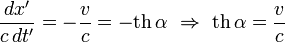
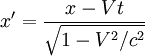
In classical kinematics, the total displacement x in the R frame is the sum of the relative displacement x′ in frame R’ and of the distance between the two origins x-x’. If v is the relative velocity of R’ relative to R, we have v: x = x′ + vt or x′ = x − vt. This relationship is linear for a constant v, that is when R and R’ are Galilean frames of reference.
In Einstein’s relativity, the main difference with Galilean relativity is that space is a function of time and vice-versa: t ≠ t′. The most general linear relationship is obtained with four constant coefficients, α, β, γ and v:


The Lorentz transformation becomes the Galilean transformation when β = γ = 1 and α = 0.
Speed of light independent of the velocity of the source
Light being independent of the reference frame as was shown by Michelson, we need to have x = ct if x′ = ct′. In other words, light moves at velocity c in both frames. Replacing x and x′ in the preceding equations, one has:


Replacing t′ with the help of the second equation, the first one writes:

After simplification by t and dividing by cβ, one obtains:

Principle of relativity
According to the principle of relativity, there is no privileged Galilean frame of reference. One has to find the same Lorentz transformation from frame R to R’ or from R’ to R. As in the Galilean transformation, the transport velocity has to be changed from v to -v when passing from one frame to the other.
The following derivation uses only the principle of relativity which is independent of light velocity constancy.
The inverse transformation of

is given by
- .

 .
.In accordance with the principle of relativity, the expressions of x and t are
- .

 .
.As the right hand sides have to be identical to those obtained by inverting the transformation, we have the identities, valid for any x’ and t’ :


Substituting x’=1 and t’=0 in the first identity and x’=0 and t’=1 in the second, we immediately get the equalities

Expression of the Lorentz transformation
Using the earlier obtained relation

one has

and, finally

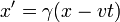
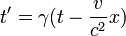
We now have all the coefficients needed and, therefore, the Lorentz transformation
- ,
![{displaystyle x={frac {x'+vt'}{sqrt[{}]{1-{frac {v^{2}}{c^{2}}}}}}}](https://wikimedia.org/api/rest_v1/media/math/render/png/c6cfa1e03eb661a981897b9e6c35c703214999d4)
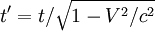
![{displaystyle t={frac {t'+{frac {vx'}{c^{2}}}}{sqrt[{}]{1-{frac {v^{2}}{c^{2}}}}}}}](https://wikimedia.org/api/rest_v1/media/math/render/png/51a92b498f3856ca7624d16158edfd9fc574ce82) ,
,or, using the Lorentz factor γ,

and its inverse:

See also
- Electromagnetic field
- Galilean transformation
- Hyperbolic rotation
- Invariance mechanics
- Lorentz group
- Principle of relativity
- Velocity-addition formula
- Algebra of physical space
- Relativistic aberration
References
- From Lorentz transformation

|
This page uses content that though originally imported from the Wikipedia article Lorentz transformation might have been very heavily modified, perhaps even to the point of disagreeing completely with the original wikipedia article. The list of authors can be seen in the page history. The text of Wikipedia is available under the Creative Commons Licence. |
A visualisation of the Lorentz transformation (full animation). Only one space coordinate is considered. The thin solid lines crossing at right angles depict the time and distance coordinates of an observer at rest with respect to that frame; the skewed solid straight lines depict the coordinate grid of an observer moving with respect to that same frame.
In physics, the Lorentz transformation describes how, according to the theory of special relativity, two observers’ varying measurements of space and time can be converted into each other’s frames of reference. It is named after the Dutch physicist Hendrik Lorentz. It reflects the surprising fact that observers moving at different velocities may measure different distances, elapsed times, and even different orderings of events.
The Lorentz transformation was originally the result of attempts by Lorentz and others to explain how the speed of light was observed to be independent of the reference frame, and to understand the symmetries of the laws of electromagnetism. Albert Einstein later re-derived the transformation from his postulates of special relativity. The Lorentz transformation supersedes the Galilean transformation of Newtonian physics, which assumes an absolute space and time (see Galilean relativity). According to special relativity, this is a good approximation only at relative speeds much smaller than the speed of light.
If space is homogeneous, then the Lorentz transformation must be a linear transformation. Also, since relativity postulates that the speed of light is the same for all observers, it must preserve the spacetime interval between any two events in Minkowski space. The Lorentz transformation describes only the transformations in which the spacetime event at the origin is left fixed, so they can be considered as a hyperbolic rotation of Minkowski space. The more general set of transformations that also includes translations is known as the Poincaré group.
Lorentz transformation for frames in standard configuration
Standard configuration of coordinate systems for Lorentz transformations.
Assume there are two observers O and Q, each using their own Cartesian coordinate system to measure space and time intervals. O uses and Q uses . Assume further that the coordinate systems are oriented so that the x-axis and the x’ -axis are collinear, the y-axis is parallel to the y’ -axis, as are the z-axis and the z’ -axis. The relative velocity between the two observers is v along the common x-axis. Also assume that the origins of both coordinate systems are the same. If all these hold, then the coordinate systems are said to be in standard configuration. A
symmetric presentation
between the forward Lorentz Transformation and the inverse Lorentz Transformation
can be achieved if coordinate systems are in
symmetric configuration.
The symmetric form highlights that all physical laws should be of such a kind that
they remain unchanged under a Lorentz transformation.
The Lorentz transformation for frames in standard configuration can be shown to be:
where is called the Lorentz factor.
Matrix form
This Lorentz transformation is called a «boost» in the x-direction and is often expressed in matrix form as
This transformation matrix is universal for all four-vectors.
More generally for a boost in any arbitrary direction ,
where and .
Note that this transformation is only the «boost,» i.e., a transformation between two frames whose , and axis are parallel and whose spacetime origins coincide (see The «Standard configuration» Figure). The most general proper Lorentz transformation also contains a rotation of the three axes, because the composition of two boosts is not a pure boost but is a boost followed by a rotation. The rotation gives rise to Thomas precession. The boost is given by a symmetric matrix, but the general Lorentz transformation matrix need not be symmetric.
The composition of two Lorentz boosts B(u) and B(v) of velocities u and v is given by:
- ,
where uv is the velocity-addition, and Gyr[u,v] is the rotation arising from the composition, gyr being the gyrovector space abstraction of the gyroscopic Thomas precession, and B(v) is the 4×4 matrix that uses the components of v, i.e. v1, v2, v3 in the entries of the matrix, or rather the components of v/c in the representation that is used above.
The composition of two Lorentz transformations L(u,U) and L(v,V) which include rotations U and V is given by:
If the 3×3 matrix form of the rotation applied to spatial coordinates is given by gyr[u,v], then the 4×4 matrix rotation applied to 4-coordinates is given by:
- .
Views of spacetime along the world line of a rapidly accelerating observer (center) moving in a 1-dimensional (straight line) «universe». The vertical direction indicates time, while the horizontal indicates distance, the dashed line is the spacetime trajectory («world line») of the observer. The small dots are specific events in spacetime. If one imagines these events to be the flashing of a light, then the events that pass the two diagonal lines in the bottom half of the image (the past light cone of the observer in the origin) are the events visible to the observer. The slope of the world line (deviation from being vertical) gives the relative velocity to the observer. Note how the view of spacetime changes when the observer accelerates.![]()
For a boost in an arbitrary direction with velocity , it is convenient to decompose the spatial vector into components perpendicular and parallel to the velocity : . Then only the component in the direction of is ‘warped’ by the gamma factor:
where now . The second of these can be written as:
These equations can be expressed in matrix form as
where I is the identity matrix, v is velocity written as a column vector, vT is its transpose (a row vector) and is its versor.
Rapidity
The Lorentz transformation can be cast into another useful form by defining a parameter called the rapidity (an instance of hyperbolic angle) such that
so that
Equivalently:
Then the Lorentz transformation in standard configuration is:
Hyperbolic trigonometric expressions
From the above expressions for eφ and e−φ
and therefore,
Hyperbolic rotation of coordinates
Substituting these expressions into the matrix form of the transformation, we have:
Thus, the Lorentz transformation can be seen as a hyperbolic rotation of coordinates in Minkowski space, where the rapidity represents the hyperbolic angle of rotation, often referred to as rapidity.
Lorentz transformation of the electromagnetic field
The fact that the electromagnetic field shows relativistic effects becomes clear by carrying out a simple thought experiment:
- Consider an observer looking at a charge being at rest. The observer will find out that there is an electric field. Since there is no electric current, however, he will state not seing any magnetic field.
- If the observer moves toward or away from the charge with a certain velocity , he will notice that the electric field changes its value as a result of motion. This means, that he will measure different electric fields at the same place, depending on whether he is at motion or not. On the other hand, the observer will interpret the charge at motion as an electric current having a magnetic field around it.
This shows that electromagnetic field quantities need to undergo a Lorentz transformation when changing the frame of reference.
For the electric and magnetic field quantities, the following transformations apply :
In non-relativistic approximation, i. e. for speeds , the relativistic factor equals , so that there is no need to distinguish between the spatial and temporal coordinates in Maxwell’s equations. This yields the following transformations:
The electric and magnetic fields transform differently from space and time, but exactly the same way as relativistic angular momentum and the boost vector.
The electromagnetic field strength tensor is given by
in SI units. In relativity, the Gaussian system of units is often preferred over SI units, even in texts whose main choice of units is SI units, because in it the electric field E and the magnetic induction B have the same units making the appearance of the electromagnetic field tensor more natural. Consider a Lorentz boost in the x-direction. It is given by
where the field tensor is displayed side by side for easiest possible reference in the manipulations below.
The general transformation law (T3) becomes
For the magnetic field one obtains
For the electric field results
Here, β = (β, 0, 0) is used. These results can be summarized by
and are independent of the metric signature. For SI units, substitute E → E⁄c. Misner, Thorne & Wheeler (1973) refer to this last form as the 3 + 1 view as opposed to the geometric view represented by the tensor expression
and make a strong point of the ease with which results that are difficult to achieve using the 3 + 1 view can be obtained and understood. Only objects that have well defined Lorentz transformation properties (in fact under any smooth coordinate transformation) are geometric objects. In the geometric view, the electromagnetic field is a six-dimensional geometric object in spacetime as opposed to two interdependent, but separate, 3-vector fields in space and time. The fields E (alone) and B (alone) do not have well defined Lorentz transformation properties. The mathematical underpinnings are equations (T1) and (T2) that immediately yield (T3). One should note that the primed and unprimed tensors refer to the same event in spacetime. Thus the complete equation with spacetime dependence is
Length contraction has an effect on charge density ρ and current density J, and time dilation has an effect on the rate of flow of charge (current), so charge and current distributions must transform in a related way under a boost. It turns out they transform exactly like the space-time and energy-momentum four-vectors,
or, in the simpler geometric view,
Spacetime interval
In a given coordinate system (), if two events and are separated by
the spacetime interval between them is given by
This can be written in another form using the Minkowski metric. In this coordinate system,
Then, we can write
or, using the Einstein summation convention,
Now suppose that we make a coordinate transformation . Then, the interval in this coordinate system is given by
or
It is a result of special relativity that the interval is an invariant. That is, . It can be shown that this requires the coordinate transformation to be of the form
Here, is a constant vector and a constant matrix, where we require that
Such a transformation is called a Poincaré transformation or an inhomogeneous Lorentz transformation. The represents a spacetime translation. When , the transformation is called an homogeneous Lorentz transformation, or simply a Lorentz transformation.
Taking the determinant of gives us
Lorentz transformations with form a subgroup called proper Lorentz transformations which is the special orthogonal group . Those with are called improper Lorentz transformations which is not a subgroup, as the product of any two improper Lorentz transformations will be a proper Lorentz transformation. From the above definition of it can be shown that , so either or , called orthochronous and non-orthochronous respectively. An important subgroup of the proper Lorentz transformations are the proper orthochronous Lorentz transformations which consist purely of boosts and rotations. Any Lorentz transform can be written as a proper orthochronous, together with one or both of the two discrete transformations; space inversion () and time reversal (), whose non-zero elements are:
The set of Poincaré transformations satisfies the properties of a group and is called the Poincaré group. Under the Erlangen program, Minkowski space can be viewed as the geometry defined by the Poincaré group, which combines Lorentz transformations with translations. In a similar way, the set of all Lorentz transformations forms a group, called the Lorentz group.
A quantity invariant under Lorentz transformations is known as a Lorentz scalar.
Special relativity
One of the most astounding consequences of Einstein’s clock-setting method is the idea that time is relative. In essence, each observer’s frame of reference is associated with a unique set of clocks, the result being that time passes at different rates for different observers. This was a direct result of the Lorentz transformations and is called time dilation. We can also clearly see from the Lorentz «local time» transformation that the concept of the relativity of simultaneity and of the relativity of length contraction are also consequences of that clock-setting hypothesis.
Lorentz transformations can also be used to prove that magnetic and electric fields are simply different aspects of the same force — the electromagnetic force. If we have one charge or a collection of charges which are all stationary with respect to each other, we can observe the system in a frame in which there is no motion of the charges. In this frame, there is only an «electric field». If we switch to a moving frame, the Lorentz transformation will predict that a «magnetic field» is present. This field was initially unified in Maxwell’s concept of the «electromagnetic field».
The correspondence principle
For relative speeds much less than the speed of light, the Lorentz transformations reduce to the Galilean transformation in accordance with the correspondence principle.
The correspondence limit is usually stated mathematically as: as , . In words: as velocity approaches 0, the speed of light (seems to) approach infinity. Hence, it is sometimes said that nonrelativistic physics is a physics of «instant action at a distance».
History
- See also History of Lorentz transformations.
Many physicists, including George FitzGerald, Joseph Larmor, Hendrik Lorentz and Woldemar Voigt, had been discussing the physics behind these equations since 1887.
Larmor and Lorentz, who believed the luminiferous ether hypothesis, were seeking the transformation under which Maxwell’s equations were invariant when transformed from the ether to a moving frame. Early in 1889, Oliver Heaviside had shown from Maxwell’s equations that the electric field surrounding a spherical distribution of charge should cease to have spherical symmetry once the charge is in motion relative to the ether. FitzGerald then conjectured that Heaviside’s distortion result might be applied to a theory of intermolecular forces. Some months later, FitzGerald published his conjecture in Science to explain the baffling outcome of the 1887 ether-wind experiment of Michelson and Morley. This idea was extended by Lorentz
and Larmor
over several years, and became known as the FitzGerald-Lorentz explanation of the Michelson-Morley null result, known early on through the writings of Lodge, Lorentz, Larmor, and FitzGerald.
Their explanation was widely known before 1905.
Larmor is also credited to have been the first to understand the crucial time dilation property inherent in his equations.
In 1905, Henri Poincaré was the first to recognize that the transformation has the properties of a mathematical group,
and named it after Lorentz.
Later in the same year Einstein derived the Lorentz transformation under the assumptions of the principle of relativity and the constancy of the speed of light in any inertial reference frame,
obtaining results that were algebraically equivalent to
Larmor’s (1897) and Lorentz’s (1899, 1904), but with a different interpretation.
Paul Langevin (1911) said of the transformation:
- «It is the great merit of H. A. Lorentz to have seen that the fundamental equations of electromagnetism admit a group of transformations which enables them to have the same form when one passes from one frame of reference to another; this new transformation has the most profound implications for the transformations of space and time».
Derivation
The usual treatment is based on the invariance of the speed of light, as seen by the Michelson-Morley experiment. However, this is not necessarily the starting point: indeed (as is exposed, for example, in the second volume of the Course of Theoretical Physics by Landau and Lifshitz), what is really at stake is the locality of interactions: one supposes that the influence that one particle, say, exerts on another can not be transmitted instantaneously. Hence, there exists a theoretical maximal speed of information transmission which must be invariant, and it turns out that this speed coincides with the speed of light in vacuum. The need for locality in physical theories was already noted by Newton (see Koestler’s The Sleepwalkers), who considered the notion of an action at a distance «philosophically absurd» and believed that gravity must be transmitted by an agent (such as an interstellar aether) which obeys certain physical laws.
Michelson and Morley in 1887 designed an experiment, employing an interferometer and a half-silvered mirror, that was accurate enough to detect aether flow. The mirror system reflected the light back into the interferometer. If there were an aether drift, it would produce a phase shift and a change in the interference that would be detected. However, no phase shift was ever found. The negative outcome of the Michelson-Morley experiment left the concept of aether (or its drift) undermined. There was consequent perplexity as to why light evidently behaves like a wave, without any detectable medium through which wave activity might propagate.
In a 1964 paper, Erik Christopher Zeeman showed that the causality preserving property, a condition that is weaker in a mathematical sense than the invariance of the speed of light, is enough to assure that the coordinate transformations are the Lorentz transformations.
From group postulates
Following is a classical derivation (see, e.g., [1] and references therein) based on group postulates and isotropy of the space.
Coordinate transformations as a group
The coordinate transformations between inertial frames form a group (called the proper Lorentz group) with the group operation being the composition of transformations (performing one transformation after another). Indeed the four group axioms are satisfied:
- Closure: the composition of two transformations is a transformation: consider a composition of transformations from the inertial frame to inertial frame , (denoted as ), and then from to inertial frame , , there exists a transformation, , directly from an inertial frame to inertial frame .
- Associativity: the result of and is the same, .
- Identity element: there is an identity element, a transformation .
- Inverse element: for any transformation there exists an inverse transformation .
Transformation matrices consistent with group axioms
Let us consider two inertial frames, K and K’, the latter moving with velocity with respect to the former. By rotations and shifts we can choose the z and z’ axes along the relative velocity vector and also that the events (t=0,z=0) and (t’=0,z’=0) coincide. Since the velocity boost is along the z (and z’) axes nothing happens to the perpendicular coordinates and we can just omit them for brevity. Now since the transformation we are looking after connects two inertial frames, it has to transform a linear motion in (t,z) into a linear motion in (t’,z’) coordinates. Therefore it must be a linear transformation. The general form of a linear transformation is
where and are some yet unknown functions of the relative velocity .
Let us now consider the motion of the origin of the frame K’. In the K’ frame it has coordinates (t’,z’=0), while in the K frame it has coordinates (t,z=vt). These two points are connected by our transformation
from which we get
- .
Analogously, considering the motion of the origin of the frame K, we get
from which we get
- .
Combining these two gives and the transformation matrix has simplified a bit,
Now let us consider the group postulate inverse element. There are two ways we can go from the coordinate system to the coordinate system. The first is to apply the inverse of the transform matrix to the coordinates:
The second is, considering that the coordinate system is moving at a velocity relative to the coordinate system, the coordinate system must be moving at a velocity relative to the coordinate system. Replacing with in the transformation matrix gives:
Now the function can not depend upon the direction of because it is apparently the factor which defines the relativistic contraction and time dilation. These two (in an isotropic world of ours) cannot depend upon the direction of . Thus, and comparing the two matrices, we get
According to the closure group postulate a composition of two coordinate transformations is also a coordinate transformation, thus the product of two of our matrices should also be a matrix of the same form. Transforming to and from to gives the following transformation matrix to go from to :
In the original transform matrix, the main diagonal elements are both equal to , hence, for the combined transform matrix above to be of the same form as the original transform matrix, the main diagonal elements must also be equal. Equating these elements and rearranging gives:
The denominator will be nonzero for nonzero v as is always nonzero, as . If v=0 we have the identity matrix which coincides with putting v=0 in the matrix we get at the end of this derivation for the other values of v, making the final matrix valid for all nonnegative v.
For the nonzero v, this combination of function must be a universal constant, one and the same for all inertial frames. Let’s define this constant as where has the dimension of . Solving
we finally get and thus the transformation matrix, consistent with the group axioms, is given by
If were positive, then there would be transformations (with ) which transform time into a spatial coordinate and vice versa. We exclude this on physical grounds, because time can only run in the positive direction. Thus two types of transformation matrices are consistent with group postulates: i) with the universal constant and ii) with .
Galilean transformations
If then we get the Galilean-Newtonian kinematics with the Galilean transformation,
where time is absolute, , and the relative velocity of two inertial frames is not limited.
Lorentz transformations
If is negative, then we set which becomes the invariant speed, the speed of light in vacuum. This yields and thus we get special relativity with Lorentz transformation
where the speed of light is a finite universal constant determining the highest possible relative velocity between inertial frames.
If the Galilean transformation is a good approximation to the Lorentz transformation.
Only experiment can answer the question which of the two possibilities, or , is realised in our world. The experiments measuring the speed of light, first performed by a Danish physicist Ole Rømer, show that it is finite, and the Michelson–Morley experiment showed that it is an absolute speed, and thus that .
From physical principles
The problem is usually restricted to two dimensions by using a velocity along the x axis such that the y and z coordinates do not intervene. It is similar to that of Einstein. More details may be found in
As in the Galilean transformation, the Lorentz transformation is linear : the relative velocity of the reference frames is constant. They are called inertial or Galilean reference frames. According to relativity no Galilean reference frame is privileged. Another condition is that the speed of light must be independent of the reference frame, in practice of the velocity of the light source.
Galilean reference frames
In classical kinematics, the total displacement x in the R frame is the sum of the relative displacement x′ in frame R’ and of the distance between the two origins x-x’. If v is the relative velocity of R’ relative to R, we have v: x = x′ + vt or x′ = x − vt. This relationship is linear for a constant v, that is when R and R’ are Galilean frames of reference.
In Einstein’s relativity, the main difference with Galilean relativity is that space is a function of time and vice-versa: t ≠ t′. The most general linear relationship is obtained with four constant coefficients, α, β, γ and v:
The Lorentz transformation becomes the Galilean transformation when β = γ = 1 and α = 0.
Speed of light independent of the velocity of the source
Light being independent of the reference frame as was shown by Michelson, we need to have x = ct if x′ = ct′. In other words, light moves at velocity c in both frames. Replacing x and x′ in the preceding equations, one has:
Replacing t′ with the help of the second equation, the first one writes:
After simplification by t and dividing by cβ, one obtains:
Principle of relativity
According to the principle of relativity, there is no privileged Galilean frame of reference. One has to find the same Lorentz transformation from frame R to R’ or from R’ to R. As in the Galilean transformation, the transport velocity has to be changed from v to -v when passing from one frame to the other.
The following derivation uses only the principle of relativity which is independent of light velocity constancy.
The inverse transformation of
is given by
- .
In accordance with the principle of relativity, the expressions of x and t are
- .
As the right hand sides have to be identical to those obtained by inverting the transformation, we have the identities, valid for any x’ and t’ :
Substituting x’=1 and t’=0 in the first identity and x’=0 and t’=1 in the second, we immediately get the equalities
Expression of the Lorentz transformation
Using the earlier obtained relation
one has
and, finally
We now have all the coefficients needed and, therefore, the Lorentz transformation
- ,
or, using the Lorentz factor γ,
and its inverse:
See also
- Electromagnetic field
- Galilean transformation
- Hyperbolic rotation
- Invariance mechanics
- Lorentz group
- Principle of relativity
- Velocity-addition formula
- Algebra of physical space
- Relativistic aberration
References
- From Lorentz transformation
|
|
This page uses content that though originally imported from the Wikipedia article Lorentz transformation might have been very heavily modified, perhaps even to the point of disagreeing completely with the original wikipedia article. The list of authors can be seen in the page history. The text of Wikipedia is available under the Creative Commons Licence. |
Преобразования Лоренца
2006-10-22 02:07
Преобразования Лоренца
Пусть нам даны две системы отсчета k и k`. В момент t = О обе
эти системы координат совпадают. Пусть система k` (назовем ее
подвижной) движется так, что ось х` скользит по оси х, ось у`
параллельна оси у, скорость v — скорость движения этой
системы координат (рис. 109).
Точка М имеет координаты в системе k — х, у, z, a в системе k`
— х`, у`, z`.
Преобразования Галилея в классической механике имеют вид:
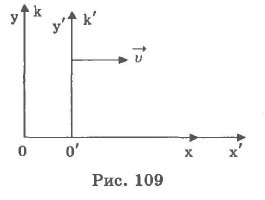
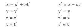
Преобразования координат, удовлетворяющие постулатам
специальной теории относительности, называются
преобразованиями Лоренца.
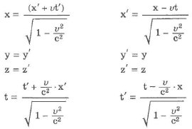
Впервые они (в несколько иной форме) были предложены Лоренцем
для объяснения отрицательного эксперимента Майкельсона-Морли и
для придания уравнениям Максвелла одинакового вида во всех
инерциальных системах отсчета.
Эйнштейн вывел их независимо на основе своей теории
относительности. Подчеркнем, что изменилась (по сравнению с
преобразованием Галилея) не только формула преобразования
координаты х, но и формула преобразований времени t. Из
последней формулы непосредственно видно, как переплетены
пространственная и временная координаты.
Следствия из преобразований Лоренца
-
Длина движущегося стержня.
Предположим, что стержень расположен вдоль оси х` в
системе k` и движется вместе с системой k` со
скоростью v.Разность между координатами конца и начала отрезка в
системе отсчета, в которой он неподвижен, называется
собственной длиной отрезка. В нашем случае
l0 = х2` —
х1`, где х2` — координата конца
отрезка в системе k` и х/ — координата начала.
Относительно системы k стержень движется. Длиной
движущегося стержня принимают разность между
координатами конца и начала стержня в один и тот же
момент времени по часам системы k.
где l — длина движущегося стержня, l0
— собственная длина стержня. Длина движущегося стержня
меньше собственной длины. -
Темп хода движущихся часов.
Пусть в точке х0` движущейся системы
координат k` происходит последовательно два события в
моменты t/ и t2. В неподвижной системе
координат k эти события происходят в разных точках в
моменты t1 и t2. Интервал
времени между этими событиями в движущейся системе
координат равен дельта t` = t2` —
t1`, а в покоящейся дельта t =
t2 — t1.На основании преобразования Лоренца получим:

Интервал времени дельта t` между событиями, измеренный
движущимися часами, меньше, чем интервал времени
дельта t между теми же событиями, измеренный
покоящимися часами. Это означает, что темп хода
движущихся часов замедлен относительно неподвижных.Время, которое измеряется по часам, связанным с
движущейся точкой, называется собственным
временем этой точки. -
Относительность одновременности.
Из преобразований Лоренца следует, что если в системе
k в точке с координатами x1 и х2
происходили два события одновременно (t1 =
t2 = t0), то в системе k`
интервал
понятие одновременности — понятие относительное.
События, одновременные в одной системе координат,
оказались неодновременными в другой. -
Относительность одновременности и причинность.
Из относительности одновременности следует, что
последовательность одних и тех же событий в различных
системах координат различна.Не может ли случиться так, что в одной системе
координат причина предшествует следствию, а в другой,
наоборот, следствие предшествует причине?Чтобы причинно-следственная связь между событиями
имела объективный характер и не зависела от системы
координат, в которой она рассматривается, необходимо,
чтобы никакие материальные воздействия, осуществляющие
физическую связь событий, происходящих в различных
точках, не могли передаваться со скоростью, большей
скорости света.Таким образом, передача физического влияния из одной
точки в другую не может происходить со скоростью,
большей скорости света. При этом условии причинная
связь событий носит абсолютный характер: не существует
системы координат, в которой причина и следствие
меняются местами.
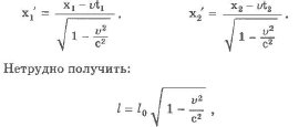
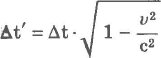
Видео
-

Физика воздуха. Сжимаемость воздуха.
2020-05-23
-
Что такое электричество? | ПРОСТО ФИЗИКА с Алексеем Иванченко
2020-05-23
-
Курс подготовки к ЕГЭ. Физика. Урок №1 Кинематика равномерного движения
2018-12-22
-
Батавские слезки — опыты
2017-12-15
-
Тепловой рычаг — физические опыты
2017-12-15
-
Секрет ЖК-монитора — поляризационная пленка
2017-12-15
-
ЛАЗЕР В ВОДЕ — физические опыты
2017-12-15
-
ЭЛЕКТРОХРОМНАЯ ПЛЕНКА с токопроводящим слоем и жидкокристаллической основой
2017-12-15
-
Урок из космоса.Физика невесомости
2017-12-12
-
Абсолютный ноль — погоня за абсолютным нулём
2017-12-12


Преобразования Лоренца — математические преобразования в специальной теории относительности, которым подвергаются галилеевы координаты события при переходе от одной инерциальной системы отсчёта (ИСО) — к другой. Образуют группу — так называемую группу Пуанкаре.
Иногда под преобразованиями Лоренца понимают только частный случай преобразований: от одной ИСО к другой, когда начала отсчёта обоих ИСО совпадают. Эти преобразования также образуют группу — группу Лоренца, которая является подгруппой группы Пуанкаре.
Вид преобразований при коллинеарных осях
Если ИСО K’ движется относительно ИСО K с постоянной скоростью  вдоль оси
  , а начала координат совпадают в начальный момент времени в обеих системах, то преобразования Лоренца (обратные) имеют вид:
 ,
,
где  — скорость света в вакууме.
Формулы, выражающие обратное преобразование, то есть,  через
через  можно получить заменой на
  .
.
Вид преобразований при произвольной ориентации осей
В силу произвольности введения осей координат, многие задачи можно свести к указанному случаю. Если же задача требует иного расположения осей, то можно воспользоваться формулами преобразований в более общем случае. Для этого радиус-вектор точки
 ,
,
где  — орты, надо разбить на составляющую
  параллельную скорости и составляющую
  ей перпендикулярную
 .
.
Тогда преобразования получат вид
 ,
,
где  — абсолютная величина скорости,
 — абсолютная величина продольной составляющей радиус-вектора.
Эти формулы для случая параллельных осей, но с произвольно направленной скоростью, можно преобразовать к виду, впервые полученному Герглоцем:
 ,
,
 .
.
Обратите внимание, что самый общий случай, когда начала координат не совпадают в нулевой момент времени, здесь не приведён с целью экономии места. Его можно получить, добавив к преобразованиям Лоренца линейные преобразования.
Преобразования Лоренца в матричном виде
Для случая коллинеарных осей преобразования Лоренца записываются в виде
 ,
,
где  .
.
Свойства преобразований Лоренца
Можно заметить, что в случае, когда , преобразования Лоренца переходят в преобразования Галилея. То же самое происходит в случае, когда  . Это говорит о том, что специальная теория относительности совпадает с механикой Ньютона либо в мире с бесконечной скоростью света, либо при скоростях, малых по сравнению со скоростью света. Последее объясняет, каким образом сочетаются эти две теории — первая является уточнением второй.
Связанные определения
Лоренц-инвариантность — свойство физических законов записываться одинаково во всех инерциальных системах отсчета(с учетом преобразований Лоренца). Принято считать, что этим свойством должны обладать все физические законы. Однако некоторые теории, например квантовую механику, пока не удается построить так, чтобы выполнялась Лоренц-инвариантность.
История
Преобразования названы в честь их первооткрывателя — Х. А. Лоренца, который вывел их, чтобы устранить противоречия между электродинамикой и механикой Ньютона. В 1900 г. он обнаружил, что эти преобразования оставляют инвариантными уравнения Максвелла. Сам Лоренц верил в светоносный эфир и только Эйнштейн в своей теории относительности пришёл к современной трактовке этих преобразований.
Преобразования Лоренца были впервые опубликованы в 1904 г. но в то время их форма была несовершенна. К современному, полностью самосогласованному виду их привёл французский математик А. Пуанкаре.
Литература
Ф. И. Фёдоров. Группа Лоренца. М.: Наука, 1979. 384 с.
ar:تحويلات لورينتز
ca:Transformació de Lorentz
cs:Lorentzova transformace
da:Lorentz-transformation
el:Μετασχηματισμοί Λόρεντζ
et:Lorentzi teisendused
fa:تبدیلات لورنتس
gl:Transformación de Lorentz
he:טרנספורמציות לורנץ
nl:Lorentztransformatie
pl:Transformacja Lorentza
sk:Lorentzova transformácia
sl:Lorentzova transformacija
sv:Lorentztransformation
uk:Перетворення Лоренца